February 19, 2021
Typically we discretize continuous functions to make them tractable. For example, when representing a probability distribution, one creates discrete bins of a fixed granularity, and assigns a probability to each such that (reduce + bins) is ~1.
Consequently, programmers are very good at discretizing continuous mathematics. But the inverse is also valuable!
Sigmoid functions are good for elegantly describing some intuitions that might otherwise be clumsily represented with prolific branching. Specifically, intuitions of the “gradually, then suddenly” variety.
By intuition I mean something like: you’re a market maker buying and selling an asset, and if you were controlling things manually you’d bias your trading long (you think it’s going up!), but at the same time if the market is selling to you too eagerly, you might get the feeling that you should back off a bit (what do they know that you don’t?), not completely closing out your position, but buying slightly less enthusiastically and selling a little more aggressively, to flatten your exposure.
Since you’re constantly buying and selling, at any given time you might be short a couple hundred or long a couple hundred, depending on a lot of fuzzy and entropic factors that you generally don’t think that much about (or at least when you do, only in aggregate). You normally just course correct by raising or lowering prices a tiny bit when you want to increase your likelihood of buying or selling to correct back towards your position target, unless you start to “feel” like something is off, in which case you take more aggressive action.
A discrete algorithm might:
- Define some position threshold for “abnormal”, e.g. exceeding +/- 200.
- Define some normal price change increment, and scale it in proportion to position size while inside of the normal range, adding a positive constant shift to introduce a long bias.
- Define an agressive price change increment, and scale it in proportion to position size while outside of the normal range.
- Iterate on this dynamic, creating more thresholds and price increments as necessary to approximate the MM’s intuition in “normal”, “medium-weird”, and “crazy” situations.
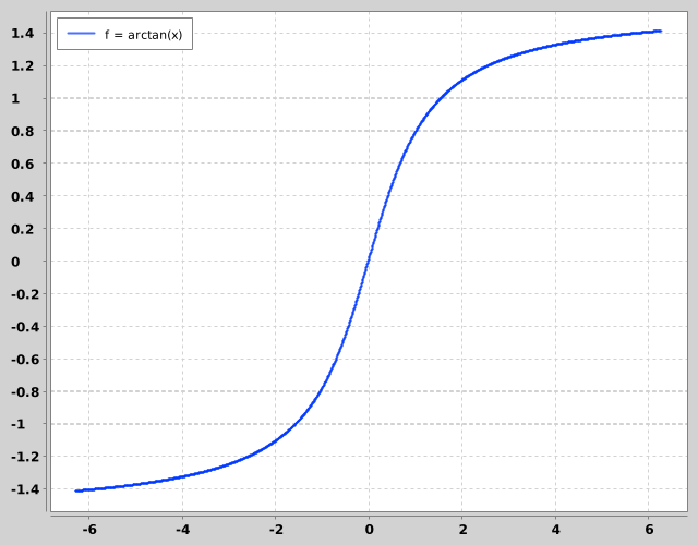
A continuous approach produces a better model: use something like arctan(x), mapped onto a domain of possible position sizes, and a range of possible price adjustments. Center the domain around a slightly positive number (to introduce your long bias), and you’re good to go.
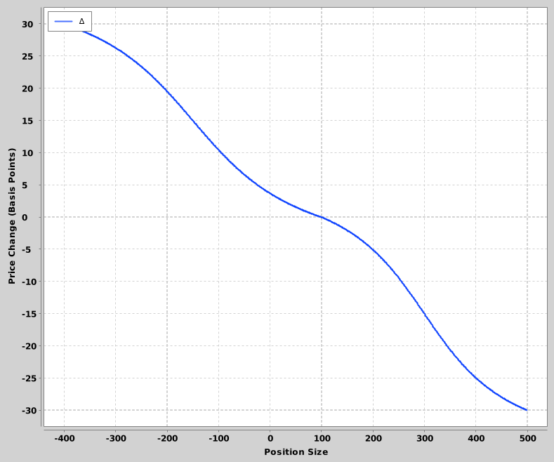
On either side of the slightly positive bias (x = 100) is arctangent over -π to +π, transformed to fit some range of positions (-400 to +100 on the left, +100 to +500 on the right) and arbitrary price skews from +0.0030% to -0.0030%.
Whether this lovely distillation of the “gradually, then suddenly” intuition is enough to turn a profit is a separate question!
You can even capture some particular “temperament” of response — map from arctangent domains sized π vs 2π or 3π for relatively cool-headed and hot-headed responses.
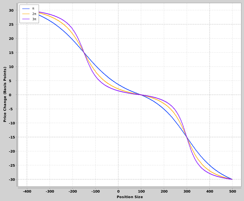
The implementation might even be smaller, and more general.
;; The basic shape of the sigmoid function
(defn atan'
  "Arctangent, but squished onto a field where x, y ∈ [0, 1]."
  [atan-domain]
  (let [shift (/ atan-domain 2)
        y-shift (Math/atan shift)
        y-range (* 2 y-shift)]
    (fn s-curve [x]
      (/ (+ (Math/atan (* (- x 0.5) atan-domain)) y-shift) y-range))))

;; Map any 1x1 curve shape onto a differently shaped field
(defn onto-field [f & {:keys [domain range]}]
  (let [[min-x max-x] domain
        [min-y max-y] range]
    (fn [x]
      (let [x-% (/ (- x min-x) (- max-x min-x)) ; % through f's domain
            y-% (f x-%)] ; proportionate % through f's range
        (+ (* y-% (- max-y min-y)) min-y)))))

;; Functions for the left & right hand sides of the chart, corresponding to the
;; position sizes to compute price skew for.
(onto-field (atan' Math/PI) :domain [-400 +100] :range [+30 0])
(onto-field (atan' Math/PI) :domain [+100 +500] :range [0 -30])
Not only is this model’s chart satisfyingly more squiggly than that of discrete model, it also works much better (in markets with price-sensitive participants, anyway). I find this pretty cool — and it’s hard not to wonder if there are other situations where transcribing the intuition behind an algorithm is actually easier than just switching over several inflection points.
However: caution in domains with low signal to noise ratios. See Ernie Chan, and uhm, Ernest Hemingway, on bankruptcy and nonlinear models.