The Kelly criterion has always interested me, in part, because even the academic literature obsesses over the difference between theory and practice.

The Kelly criterion finds the bet size to maximize growth over a series of bets. I won’t introduce it in detail, since others have already done so (see here, here and here).

Never an armchair risk-taker, when E.O. Thorp was working on these ideas, he started by counting cards and wagering on equines before generalizing, and formalized the approach of betting less than the theoretical optimum. Common sense agrees. This is called “fractional Kelly” generally or “half Kelly” when betting exactly half the optimal amount.

I started simulating these kinds of bets, interested in something like: what properties would have to be true of ourselves and the things that we tend to bet on¹ for half Kelly to be a useful heuristic?

---

I ended up simulating a few things in turn:

1. Uncertainty. What happens if the winning probability changes with each bet according to some level of uncertainty?
2. Risk of ruin. How does a small risk of losing the entire wager affect the optimal bet size when considering only modest gains or losses as the other outcomes?
3. Downside risk mitigation. Is there a revealed preference not to maximize growth rate, but to maximize lower-than-median percentile returns?

These topics have been covered in (perhaps too much) depth in the literature, and in bits and pieces on blogs. My small addition is a series of interactive simulations to test your intuition against.

---

Uncertainty

If you bet on an outcome that you think is ~70% likely, one way to think about the winning probability is as a number drawn from a normal distribution centered around 70%, with some standard deviation, say 5%.

\[p \sim \mathcal{N}(\mu = 0.70, \sigma = 0.05)\]

In which case, there is uncertainty, and, for example, 68% of the time your winning probability is between 0.65 and 0.75. For reference, the Kelly bet (f*) for 70/30 chances is 0.40, but for 65/35 it is 0.30.

If overbetting is worse than underbetting (as Thorp shows; more on that below), then increasing uncertainty reduces the optimal bet size, even if you have the right mean. This looks like a good reason for uncertainty to affect bet sizes.

But have a look at this Monte Carlo simulation of 100 portfolios, each making 100 wagers with chances of winning drawn from a normal distribution around p(win). Drag the bet size and uncertainty bars around.

---

---

Setting the uncertainty σ to 5% moves the optimal bet size from 0.40 to 0.38. At σ = 20%, it decreases to 0.36. These are relatively small moves for significant changes in uncertainty. (Click the green links to update simulation parameters.)

Uncertainty matters, but apparently not that much. Only setting σ to extremes, like 50%, produces a significant change in optimal bet size².

Thorp on uncertainty

Thorp’s explanation is that it is not primarily uncertainty, but a background tendency to overestimate the chances of winning, and therefore to overbet, which justifies a partial Kelly strategy.

He shows that overbetting is indeed worse than underbetting, and that betting half-Kelly offers protection against a negative growth rate (from overbetting) at the cost of reducing growth rate by, in this case, <= 25%.

In other words, there’s asymmetry in your favor when reducing bet size from full to half of the theoretical optimal.

---

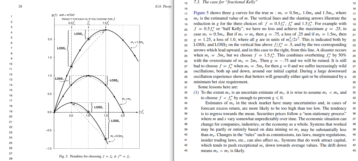
Pages 28 and 29 of “The Kelly criterion in blackjack, sports betting, and the stock market”.

---

I’m convinced that uncertainty is not as important as I thought, but only weakly convinced that the apparent usefulness of partial Kelly is due to systematic overestimation of winning probability.

Risk of ruin

If everyone were underestimating a permeating, Talebian risk of ruin, that might explain the appeal of partial Kelly betting.

Take Credit Suisse’s AT1 securities. They were bond-like things which paid a 9.75% coupon with very high probability, but they were also (apparently) the first backstop for depositors if bank capital were to become insufficient. So a bet size based on Fermi estimates of the relative value of the AT1s in different interest rate environments would require serious modification to account for even a 1% risk of going to zero.

Or take a stock whose price is 100. If you think there’s a 60/40 shot it either climbs to 125 or falls to 75, the Kelly bet size is \(f* = {0.60 \over 0.25} - {0.40 \over 0.25} = 0.8\). But factoring in a a 1% risk of ruin yields an optimal bet of 0.46³, and a 2% risk of ruin further decreases it to 0.39.

---

---

This is more persuasive. However, it depends on a combination of low assumed downside risk and proportionally small actual risk of ruin. So while I think risk of ruin is important, I’m not totally convinced it’s the main driver of the apparent usefulness of fractional Kelly strategies. Plenty of Kelly bets are made assuming a total loss in the downside case anyway, and those bettors still utilize fractional Kelly strategies.

Downside risk mitigation

Here’s another explanation: maybe our revealed preference is not to maximize the growth of the median portfolio, but to maximize the growth of the 10th percentile portfolio⁴.

In a Monte Carlo simulation of portfolios following the same strategy, the mean is important, but one’s true preference might be closer to something like “I want to follow a strategy where I’d make money in 9 / 10 hypothetical worlds”.

Take the same 70/30, even payout bet, this time optimizing for percentiles other than the 50th:

---

---

Drag the nth percentile control around. Optimizing for the 10th percentile, or the 20th, yields a very different bet size than optimizing for the 50th percentile.

Full Kelly has an interesting property: there is an X% chance of your bankroll dropping to X% of what you started with⁵. A 50% chance of a 50% drawdown is a lot to stomach. Maybe we’d rather not have optimal growth.

In his post on the Kelly criterion, Zvi notes that full Kelly is only correct if you know your edge and can handle the swings. He also notes that you don’t know your edge, and you can’t handle the swings.

This is a compelling explanation for the fractional Kelly heuristic, because it explains large downward adjustments in the bet fraction. Here too, the adjustment depends on the odds ratio, though:

• For a 70/30 bet with even payoffs, optimizing for the 10th percentile return lowers the optimal bet from 0.40 to 0.28.
• But for a 30/70 bet, where winning pays a 5x return⁶, optimizing for the 10th percentile return lowers the optimal bet from 0.13 to 0.05.

This makes sense, because the distribution of final returns has higher or lower variance depending on whether the bets have higher or lower variance.

To get a better feel for this dynamic, consider a 3d plot of optimal bet sizes for wagers with for the same expected value (EV) and different probabilities of winning, across three surfaces with different EVs.

So for example the point at p(win) = 0.75 on the 1.5 EV surface represents an even bet (you 2x your wager if you win, 0x if you lose), but at p(win) = 0.5, the odds change such that you 3x if you win, to maintain the same EV.

---

---

One way to think about the Kelly criterion is as recognition of the slope along the bet size ⇔ p(win) curve for a fixed expected value. Perhaps some part of the driving intuition behind fractional Kelly, beyond uncertainty about where one sits on the first curve, is the recognition that there is also slope along the percentile axis.⁷

Closing remarks

I came away from this downgrading the importance of pure uncertainty relative to other sources of risk, and above all, with the impression that fractional Kelly is overdetermined. Kelly betting is a fascinating topic, and I enjoyed reading about it in:

• Aaron Brown’s Red-Blooded Risk
• materials from David Aldous (short page here, long pdf here)
• Thorp’s “Kelly criterion in blackjack, sports betting, and the stock market” and “Good and bad properties of the Kelly criterion” papers
• the gambling chapter in Sanjiv Das’s online stats book
• Zvi’s introductory and follow-up posts